Take just the pick list section TXT from your sheet... remove blank lines. Import it into an Excel spreadsheet. It is "delimited" using "commas". The rest of the dialog wizard you can just OK/next to.
I'd recommend starting from the prototype, and deleting the old detail data rows so that just the title row remains. When you import the next data it will be placed in the rows following the title. The presence of the title row is crucial to the pivot table concept.
Then, highlight the complete set of cells that should be part of the table, starting from the first title cell (Quantity) and running through the last detail row cell (Grade).

Then, click on the "Insert" item on the menu bar, and push the "PivotTable" button at the left of the "Tables" group on the left side of the button bar. The selected range from your just imported will appear in the table/range area, and the "new worksheet" radio button will be pre-checked. Just push OK.
The pivot table area (shown on the left side of the presentation) will initially be empty. The pivot table field list from which you can select the values to be "spun" are shown in the upper-right. Magically, Excel knows that size, length and grade are "row labels" so if you check those items in the "choose fields to add to report" they will appear down in the "row labels" quadrant area.
And if you then check the "quantity" field, it will be placed in the "sum values" quadrant area.
And magically, on the left side, the pivot table will appear... with all of the detail row values "spun" and "totaled", and it will look like this:

This matches your sample results (except that your 2x4, 6-0-0, #2 is wrong... it should be 4, not 3 as you show):111024A Pick List
1,2x6,14-0-0,2100
2,2x6,14-0-0,1650
2,2x6,10-0-0,2100
6,2x4,16-0-0,2100
2,2x4,14-0-0,2100
1,2x4,14-0-0,#2
4,2x4,12-0-0,#2
3,2x4,6-0-0,#2
Since the table itself will be of varying length, you should then select the complete table range (starting from the first row label cell to the Grand Total number, push the Page Layout item on the Menu bar, and then push the Print Area -> Set print area item in the Page Setup group of buttons. You can experiment with printing the table, and you can also push the "additional page setup" arrow (at the right side of the "Page Setup" bar) to get additional printing options for titling as you see fit.
Should get you started.
I believe if you save your final table spreadsheet, then the next time you open it up and delete the existing data rows, and import the new data rows onto the data sheet, that the previously established and checked "row labels" and "sum items" will be all set from before, and the pivot table sheet should instantly rebuild itself with the new pick list row data. You should not have to do anything more, other than probably redefine the new print area and print it.


 Quote
Quote